


Creating a New Dashboard in Excel With the Help of Pivot Tables

Introduction
I recently came across a César Hernández González interview (see below video). He is the Assistant Volleyball Coach of at VakifBank & Korean National Team and really into performance analysis.
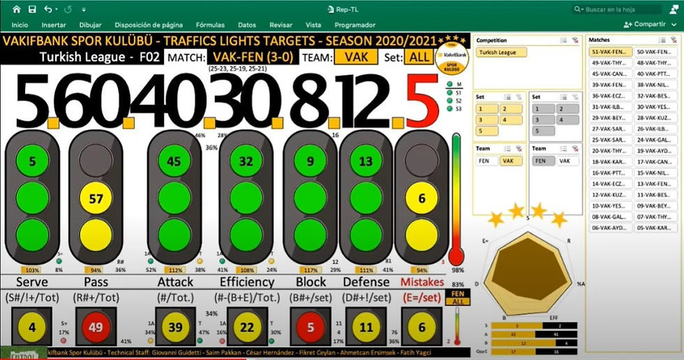
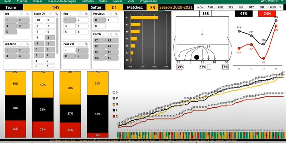
The interview was in Spanish so I had no clue what was being said. However, the dashboards he showed was beautiful (see slideshow below). Not only that, he had these panels (called slicers I later learnet) that allowed him to change the data according to match, set, player, rotation, compeition etc. I thought this interactive and dynamic spreadsheet was amazing. However, I had no clue how this was being done.


Pivot Tables and Dashboards
I audited two courses on edX.com (I went through the course material but I didn’t pay to complete the assignments to get the certificate). They were Analysing Data with Excel and Data Visualisation and Building Dashboards with Excel and Cognos. While it showed some things I already knew, it did introduce me to pivot tables. In my mind, the main difference between a regular table and a pivot table is they are dynamic. This means you can filter out certain data to get exactly what you need. For example, you can filter out the match-by-match stats to only show the match by match stats against a specific opponent. This would be useful to know when compiling your scouting report for that specific opponent. If you had a chart based on that pivot table then the chart would change accordingly too. If I was to collect that data previously, I would had to copy and paste that data into another table. So having learnt about pivot tables, I realised that was exactly how César Hernández González was able to make those tables and charts dynamic.
The course also reminded me about using data visualisation and dashboards in my analysis. Data visualisation is visualising the data in charts so people better understand what the data says. A good example is when a man uses rice to demonstrate the difference between 1 million and 1 billion and Jeff Bezos’s 122 billion (in February 2020). A dashboard, based on a car dashboard, should show you all the key information so you immediately know what you need to focus on. For example, a low fuel sensor would indicate you need to fill up your car with fuel. I have written about data visualisations and dashboards before but these two concepts has gotten away from me a little bit as I do tend to use tables, rather than charts, to demonstrate my point. I also don’t have a kick-ass dashboard that really highlights all the important information you need to start your analysis.
Creating a New Dashboard with Pivot Tables
Inspired by César Hernández González’s dashboards and wanting to learn about pivot tables, I decided I should create a brand new dashboard. I always find I learn better if I have to learn it for an actual purpose. I chose the purpose of creating some beach volleyball dashboards for the Bello brothers. They are an English beach volleyball pair competing internationally.
Below is the end result of a simple match report with a slicer to indicate which match stats is showing. The video below that shows the slicer in action and some of the other unfinished dashboards that I created. Below is the end result of a simple match report with a slicer to indicate which match stats is showing. The video below that shows the slicer in action and some of the other unfinished dashboards that I created.

Reflection
I did learn a lot during this process. They include:
Think about what data you want
How to organise that data to get the pivot table
Creating slicers, which are panels that allow you to filter out data, e.g. which matches
How to make calculations within the pivot table – it normally calculates the sum, which means the hitting percentage for the team is just the sum of the hitting percentages of the players.
You can’t actually have text or dates in the pivot table (I had a work around to get the event name and date in the dashboard)
Using a formula to modify change exported name of “01 Player Name” into “Player Name
=REPLACE(A1,1,FIND(” “,A1),””)
The use of the & function (it is amazing) to get the set scores as (20-22, 21-15, 14-16).
=”(“&AD10&”-“&AD13&”, “&AE10&”-“&AE13&IF(AF10=0,”)”,”, “&AF10&”-“&AF13&”)”)
Knowing how to change the conditioning format bars to go from right to left
Knowing how to align the conditioning format icons (basically hide the value and align like normal)
Using sparklines for the first time
Googling helps out a lot when you have a question or issue
You need some artistry to create these dashboards, something I am struggling with
Conclusion
It really took a lot of work to create that simple match dashboard. I am glad I went through the process because at least I have a basic understanding of what can be done. However, I can already see it will take so much more work if I was going to get anywhere near the dashboarding level of César Hernández González.

Comments